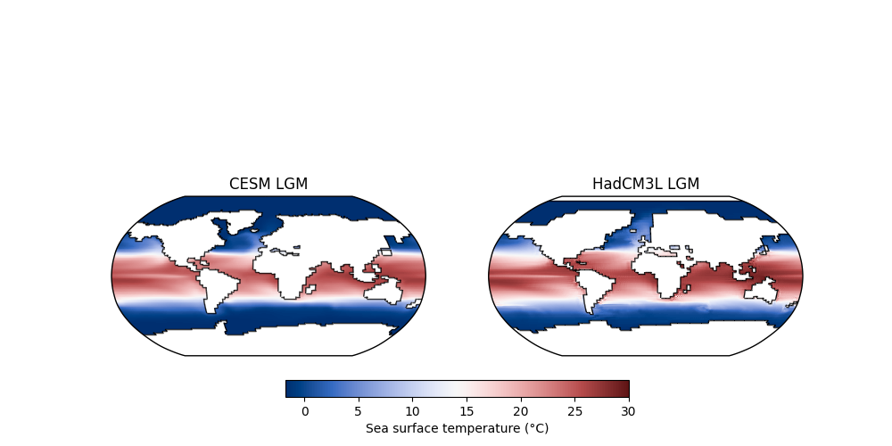
Plot Other Models’ output

This example shows how to use cgeniepy to plot gridded data from other models (CESM and HadCM3 here). You can download them from https://zenodo.org/records/13786014.

File CESM_LGM_var_regrid.nc already exists at /home/docs/.cgeniepy/CESM_LGM_var_regrid.nc. Skipping download.
Downloading teitu_020_o.pgclann.nc to /home/docs/.cgeniepy/teitu_020_o.pgclann.nc...
Download complete.

from cgeniepy.array import GriddedData
import xarray as xr
import matplotlib.pyplot as plt
import cartopy.crs as ccrs
from cgeniepy.utils import download_zenodo_file

# Define the Zenodo record and the files needed
zenodo_record_id = "13786013"
required_files = ["CESM_LGM_var_regrid.nc", "teitu_020_o.pgclann.nc"]

# Download the files
cesm_file_path = download_zenodo_file(zenodo_record_id, required_files[0])
hadcm3_file_path = download_zenodo_file(zenodo_record_id, required_files[1])

# Read in the data using the downloaded file paths
cesm_lgm = xr.load_dataset(cesm_file_path)
hadcm3_lgm = xr.load_dataset(hadcm3_file_path, decode_times=False)

# Construct GriddedData objects
cesm_temp = GriddedData(cesm_lgm['TEMP'], attrs=cesm_lgm['TEMP'].attrs)
hadcm3_temp = GriddedData(hadcm3_lgm['temp_ym_dpth'], attrs=hadcm3_lgm['temp_ym_dpth'].attrs)

# Create the plot
fig, axs = plt.subplots(1, 2, figsize=(10, 5), subplot_kw={'projection': ccrs.Robinson()})

p = cesm_temp.isel(time=0, z_t=0).to_GriddedDataVis()
p.aes_dict['pcolormesh_kwargs']['vmax'] = 30
p.plot(ax=axs[0], outline=True, colorbar=False)
axs[0].set_title('CESM LGM')

p2 = hadcm3_temp.isel(t=0, depth_1=0).to_GriddedDataVis()
p2.aes_dict['pcolormesh_kwargs']['vmax'] = 30
im = p2.plot(ax=axs[1], outline=True, colorbar=False)
axs[1].set_title('HadCM3L LGM')

fig.colorbar(im, ax=axs, orientation='horizontal', label='Sea surface temperature (°C)', fraction=0.05, pad=0.07)

plt.show()